אִם יִרְצֶה הַשֵּׁם
Li, Ma, Yang, Zhao (Peking University). arXiv:2609.03802v1 [quant-ph], 3 Sep 2026.
1. TL;DR by audience
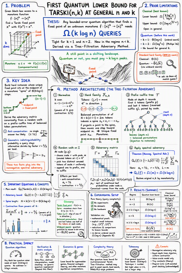
Expert (quantum complexity / TCS). First quantum lower bound for Tarski(n, k) at general n and k: Q_ε(Tarski(n,k)) = Ω(k log n), via the nonnegative spectral adversary. The hard family is a spine of Θ(k log n) monotone steps whose step vectors form a balanced permutation of tokens (direction j, scale 4^r), with the spine midpoint as unique fixed point. The adversary matrix is derived canonically from a top-down random walk on a prefix-suffix tree of token permutations; two probabilistic conditions (1/2 anti-concentration, 2/3 geometric indistinguishability) plus a block-Gram norm bound do the work. Appendix A shows the Brânzei-Phillips-Recker coordinatewise family has quantum complexity between Ω(√k / log k) and O(√k log k log n log log n) via wildcard search, so that family cannot yield a super-√k quantum bound. Tight at n = 2 and k = 1; a log n / log k gap to the classical bound remains for n ≥ k.
Practitioner (algorithm designer, verification and economics tooling). Think of a fixed point as the still point in a shifting landscape: the one state the update rule leaves alone. Finding it in a k-dimensional grid of side n costs a quantum computer at least about k · log n evaluations of the rule. For a grid of side 1024 in 100 dimensions that is a floor of roughly a thousand queries, and the naive "start at the bottom and iterate" classical method hits exactly that floor on the paper's hard instances. No quantum speedup is known for the general problem, and none is possible below k log n. If a quantum accelerator for supermodular-game equilibria or abstract-interpretation fixpoint loops was on your roadmap, this result says the black-box route has a hard floor.
General public. Many questions, from "what prices will a market settle at" to "when does this program stop changing," come down to finding a point that a rule maps back to itself. The rule is monotone: turning an input knob up never turns the output knob down. Classical computers need a known minimum number of peeks at the rule. This paper shows quantum computers face a similar minimum in high dimensions: the cost grows with the number of dimensions times the number of digits in the grid size, quantum or not. It also gives a cleaner recipe for proving such limits, by arranging hard puzzles in a 20-questions tree and walking down it at random.
Skeptic. The bound is Ω(k log n), while the best classical lower bound for n ≥ k is Ω(k log² n / log k), so in the wide-grid regime the quantum bound is weaker than what was already known classically. The gap to the best upper bound O((log n)^{(k−1)/3+1}) is enormous, so the paper says nothing about whether a quantum speedup exists. The hard family is tight for itself (iteration solves it in O(k log n)), so it cannot be pushed further. The "new method" is the standard spectral adversary with a particular matrix ansatz, demonstrated on exactly two problems, one of which (ordered search) was settled in 2001.
Decision-maker. No investment signal for quantum acceleration of fixed-point computation. This is a theoretical lower bound, publicly funded (NSFC), with no product, code, or dataset. The contribution most likely to matter beyond this problem is the proof technique, which could shorten future lower-bound proofs for tree-structured search problems.
2. The real-world problem
A monotone function on a lattice always has a fixed point (Knaster-Tarski). Computing it is the engine behind:
- Program analysis and verification. Data-flow analysis, abstract interpretation, and model checking compute least fixed points.
- Economics and game theory. Equilibria of supermodular games and clearing vectors in financial-contagion networks.
- Complexity theory. A poly(k, log n) algorithm for the grid version would put Simple Stochastic Games and Arrival into P.
The question is how many evaluations of an unknown monotone f: [n]^k → [n]^k are needed to locate a fixed point, and whether quantum query access helps. Classically the answer is open in general (upper bound about (log n)^{k/3}, lower bound about k log² n / log k). Quantumly, before this paper, only the two-dimensional case had a bound (Phillips 2026, Ω(log² n)).
3. Surprising or counterintuitive findings
- The quantum lower bound beats the classical one when n < k. For narrow grids in many dimensions, Ω(k log n) exceeds Ω(k log² n / log k). A quantum technique here yields a stronger classical statement than classical techniques had achieved.
- A standard hard family is quantumly easy. Appendix A shows the Brânzei-Phillips-Recker coordinatewise instances (classically Θ(k)) drop to about √k quantumly, up to polylog factors, via Ambainis-Montanaro wildcard search. Hardness is construction-specific, which is what forced a new family.
- The new family is tight against plain iteration. Starting from 0 and iterating f reaches the fixed point in O(k log n) steps. The lower bound cannot be improved using this family, and the authors say so.
- Powers of four, not two. Step lengths are 1, 4, 16, ... because Σ_{4^r ≤ A} 4^r ≤ (4/3)·A yields the 2/3 contraction constant. With powers of two the corresponding sum is bounded only by 2A, which gives a ratio of 1 and no contraction. A small design choice carries the whole proof.
4. Jargon decoded
| Term | Plain meaning | Concrete example |
|---|---|---|
| Tarski fixed point | A point x with f(x) = x for a function that never swaps order: bigger input, bigger-or-equal output | Prices where raising yours never lowers a competitor's best response |
| Monotone function | Turning any input knob up never turns any output knob down | A volume knob, not a light switch with a random flicker |
| Query complexity | Number of times you must ask "what is f at this point?" | Guessing a number with "higher or lower?" costs log n questions |
| Bounded-error quantum query complexity Q_ε(f) | Fewest oracle calls a quantum algorithm needs to be right with probability at least 1 − ε | Grover search finds a needle in n boxes with about √n quantum peeks instead of n |
| Nonnegative spectral adversary method | A lower-bound tool: weight pairs of inputs with different answers in a symmetric matrix; the ratio of its norm to the norm after zeroing entries a single query can tell apart bounds the query count | "Every question you ask barely dents your confusion between these pairs" |
| Distinguisher matrix Δ_i | 0/1 matrix marking which input pairs differ at position i | Which pairs of hidden numbers a single "is it above 7?" question separates |
| Spine | A monotone chain of Θ(k log n) points from the bottom corner 0 to the top corner (n−1)·1 | A staircase path through the grid |
| Token (j, r) | One spine step: move 4^r units in direction j | "Go 16 units east" |
| Balanced permutation | An ordering of tokens where the first and last halves each use half of the tokens at every scale | Ensures the spine midpoint is exactly the grid centre |
| Filtration tree | A tree whose leaves are hard instances; going down fixes more of the instance | A 20-questions tree where each level pins the next spine step at both ends |
| Simplified difference criterion D̂(u) | For a tree node u, the grid points where two instances under u could still disagree; shrinks as you descend | The region the algorithm still has reason to probe |
| Anti-concentration | Even after learning what node u reveals, no single answer has probability above 1/2 | At least two candidate fixed points always remain |
| Geometric indistinguishability | The chance a fixed query point stays informative shrinks by a constant factor per level | Probability drops like (2/3)^depth |
| Wildcard search | Quantum primitive: ask "do all bits in subset S match my guess?" and recover a k-bit string in about √k such queries | Used to break the coordinatewise hard family |
5. Methodology in detail
Step 1: Normalize parameters. Query complexity is monotone in n and k (Phillips 2026). Assume k even and n − 1 = 1 + 4 + ... + 4^U. Costs only constants.
Step 2: Build the hard family F_{n,k}. Tokens T = [k] × [U+1], N = k(U+1) = 2m tokens. A balanced permutation σ defines a spine x_0 ≺ ... ≺ x_N. The function projects a grid point v onto the spine (greatest spine vertex ≤ v if ‖v‖₁ ≤ W/2, least spine vertex ≥ v otherwise), then moves one spine index toward the midpoint m. Lemma 3.11: unique fixed point x_m. Lemma 3.12: monotone. The map σ ↦ f_σ is injective.
Step 3: Prefix-suffix tree. A node at depth t records the first t tokens and the last t tokens (reversed), constrained so paired tokens share a scale. Leaves at depth m are exactly the balanced permutations. The difference criterion at node (p, q) is the region beyond c(p) in the lower half and before B1 − c(q) in the upper half.
Step 4: Random walk. At a node, pick scale r with probability proportional to (unused tokens at scale r) × 4^r, then draw two distinct unused tokens of that scale uniformly, appending one to the prefix and one to the suffix. Lemma 4.21: conditioned on a node, the fixed point is uniform over a candidate set of size Π_r C(M_r, M_r/2), hence at least 2 (anti-concentration 1/2). Lemma 4.23: for any fixed query point x, the probability x stays in D̂ after one step is at most (4/3)(W/2 − ‖c(p)‖₁)/Z = 2/3, using Z = W − 2‖c(p)‖₁.
Step 5: Canonical adversary matrix. Γ = Σ over non-leaf nodes u of Γ_u, with Γ_u[x,y] = μ_u[x] μ_u[y] · 1{f(x) ≠ f(y)}, where μ_u is the square root of the walk's conditional leaf distribution under u. Lemma 4.12: ‖Γ‖ ≥ Σ_t a_t via the test vector v[x] = √p_x. Lemma 4.15: ‖Γ ∘ Δ_i‖ ≤ (1+√r)/(1−√r) because the per-depth matrices Q_t are orthogonal projections with ‖Q_s Q_t‖ ≤ r^{|s−t|/2} (Lemma 2.3, block-Gram argument).
Step 6: Assemble. Theorem 4.10: Q_ε(f) ≥ (1 − 2√(ε(1−ε))) · (1−√r)/(1+√r) · Σ_t a_t. With L = m, a_t = 1/2, r = 2/3 this is Ω(m) = Ω(k log n). Restore original parameters by monotonicity.
What is methodologically new. The adversary matrix is derived from a distribution rather than designed by hand. The analytic burden moves from spectral computation (the Hilbert-matrix norm in Høyer-Neerbek-Shi ordered search) to verifying two probabilistic inequalities about a random walk. Appendix B re-proves the Ω(log n) ordered-search bound this way with r = 1/2 and a_t = 1 − 2^{−(d−t)}.
6. Results with context
| Regime | This paper (quantum) | Best classical lower bound | Best upper bound | Status |
|---|---|---|---|---|
| k = 1 | Ω(log n) | Θ(log n) | O(log n) | tight (recovers HNS01) |
| n = 2, any k | Ω(k) | Θ(k) | O(k) iteration | tight (recovers BPR25a) |
| 2 ≤ k ≤ log n | Ω(k log n) | Ω(log² n) for k ≤ 4, tight there | O((log n)^{(k−1)/3+1}) | Phillips' quantum Ω(log² n) dominates |
| n < k, both ≥ 2 | Ω(k log n) | Ω(k log² n / log k) | same | new best classical and quantum bound |
| n ≥ k > log n | Ω(k log n) | Ω(k log² n / log k) | same | quantum bound trails classical by log n / log k |
| BPR25a coordinatewise family | Ω(√k / log k) ≤ Q ≤ O(√k log k log n log log n) | Θ(k) | near-quadratic quantum speedup, polylog gap open |
Explicit constant. At ε = 1/3 the prefactor is (1 − 2√2/3) · (1−√(2/3))/(1+√(2/3)) ≈ 0.0572 × 0.101 ≈ 0.0058. It multiplies Σ_t a_t = m/2 = k(U+1)/4, so the bound reads roughly 0.0014 · k(U+1). The constant is tiny and has no practical bite; the content is the order of growth.
Scale anchor. For n = 2^10 and k = 100, k log n = 1000: no quantum algorithm gets below about a thousand queries on the hard family, and plain iteration matches that on the same family.
7. Practical deployment considerations
This is pure theory; deployment means using the result or the method.
- Algorithm budgets. Any quantum Tarski solver on general grids pays at least about k log n queries. For k up to log n the classical recursive methods achieve poly(log n) already; the only room for quantum advantage is the regime where classical upper bounds are super-polylogarithmic, which is exactly where no bound of either kind exists.
- Queries are not gates. Query complexity counts oracle calls. A real implementation also pays for the oracle circuit that evaluates f, for coherence, and for error correction. A query lower bound is therefore a floor on total cost, not an estimate of it.
- Worst case, not average case. The bound holds against the paper's adversarial family. Practical instances from data-flow analysis or market models may be far easier, and iteration or coordinatewise binary search may terminate quickly on them.
- For lower-bound proofs. The Tree-Filtration recipe is checklist-like: build an equal-depth tree with a bijection to instances, define nested difference sets, exhibit a Markov walk, verify a_t and r. It should port to nested binary-search style problems (ordered search variants, poset search, local-search-style problems).
- Integration with classical results. The quantum lower bound is also a classical lower bound and supersedes BPR25b when n < k, so classical-complexity surveys should update their tables.
- Reproducibility. Proofs are self-contained. Examples 3.9 and 3.10 give small instances on [22]² and [2]⁸ that a short script can reproduce to confirm monotonicity and uniqueness.
8. Limitations, assumptions, boundary conditions
- Not tight in the main regime. For n ≥ k the classical Ω(k log² n / log k) is strictly stronger. The paper cannot close this with its own family because iteration solves it in O(k log n).
- Nonnegative adversary only. The nonnegative spectral adversary is strictly weaker than the negative-weight adversary (Høyer-Lee-Špalek 2007). Certificate-complexity style barriers may cap what this framework can prove.
- Framework restrictions. Equal-depth trees, bijective leaf map, uniform-in-depth contraction. The authors list these as open extensions.
- Value-oracle model. Results are for black-box query access. They say nothing about white-box instances given as explicit circuits, which is how fixed points arise in practice.
- Dependence on Phillips' monotonicity result. The parameter-normalization step borrows monotonicity of the complexity in n and k from Phillips 2026.
- Tiny constants. The explicit prefactor near 0.0014 has no practical meaning; only the growth rate matters.
- Novelty of the method. The abstraction resembles Ambainis' combinatorial adversary specialized to a tree; the paper itself calls it "analogous in spirit." Generality is shown on two problems, one of them a 2001 result.
9. Future directions
- Determine the quantum complexity of the multidimensional herringbone family (BPR25b); the paper flags Lemma 18 there as a candidate for a wildcard-search-style speedup.
- Build a coherent decomposition lemma (a quantum analogue of the Dang-Qi-Ye and Chen-Li recursion) to search for a genuine quantum speedup in high dimensions.
- Extend the framework: non-equal-depth trees, surjective instance maps, depth-dependent contraction, a negative-weight version.
- Apply the method to other nested-search problems: poset search, local search on graphs, monotone path following in PPAD- and PLS-style settings.
- Close the log n / log k gap, which needs a new hard family not solvable by iteration.
10. Conflicts of interest and bias flags
- Funding. NSFC Grant No. 62372006. No commercial funding disclosed.
- Citation lineage. The bibliography leans on the Brânzei/Phillips/Recker and Chen/Li line the authors extend. Normal for a narrow subfield.
- AI-assisted writing. The acknowledgement states that GPT-5.6 was used "to polishing presentation and checking the clarity and completeness of proofs." LLM proof-checking is not independent verification; treat the long arguments in Lemmas 4.14 and 4.19 as verified only by the authors. This is a v1 preprint.
- Framing. The abstract leads with "improves the best previous classical lower bound when n < k," which is true but applies to the less-studied narrow-grid regime. In the standard n ≥ k regime the result is weaker than known classical bounds; the paper states this plainly in Section 1.1 and the conclusion.
Recap
The paper proves the first quantum query lower bound Ω(k log n) for Tarski fixed points on general k-dimensional grids of side n. It is tight at the two extremes (n = 2 and k = 1) and strictly better than classical knowledge when n < k, but trails the classical Ω(k log² n / log k) when n ≥ k. It also shows the standard coordinatewise hard family admits a near-quadratic quantum speedup, and introduces a Tree-Filtration Adversary Method that derives adversary matrices from a random walk on a tree of hard instances. Main caveats: the bound is not tight in the dominant regime, the method is limited to the nonnegative adversary, and the preprint is unreviewed with LLM-assisted proof checking.